Modeling expression changes at gene level

Introduction

This vignette extends the xcore user guide by showing how to perform gene level expression modeling using RNA-seq and microarray input data.

In xcore we model the expression as a function of promoter’s sequence described by the ChIP-seq signatures. Similarly to differential expression analysis, one can consider the expression at the level of genes or transcripts. While most of the analysis steps would be identical for the two variants, the key difference is in the choice of promoters annotation. Particularly, different gene’s transcripts can have distinct promoters. One the other hand, expression at gene level is an aggregation of transcripts expression yet we would rather like to use only one promoter to describe a single gene.

xcoredata provides ChIP-seq based molecular signatures constructed against FANTOM5 promoters. These promoters correspond to transcripts’ promoters making them very easy to use with CAGE data mapped to FANTOM5 reference (as exemplified in xcore user guide). Additionally, xcoredata provides a set of core FANTOM5 promoters (promoters_f5_core) which defines only one promoter per gene. Using this core set of promoters it is possible to construct a gene level analysis with non-CAGE data, by matching input gene identifiers with core FANTOM5 promoters.

The reminder of this document shows how to construct a gene level xcore analysis. For this purpose we use publicly available RNA-seq time-series dataset obtained from classic TGFꞵ induced epithelial-to-mesenchymal transition experiment conducted in A-549 cell line (Chang H, et al. NAR. 2016., GSE69667). The other example uses microarray time-series dataset also from TGFꞵ induced epithelial-to-mesenchymal transition experiment conducted in A-549 cell line (Sartor MA, et al. Bioinformatics. 2010., GSE17708).

library("xcore")

library("xcoredata")

## snapshotDate(): 2022-10-31

RNA-seq data

Obtaining the expression data

We have downloaded the raw counts and metadata for GSE69667 study from GREIN portal that provide raw counts for many RNA-seq datasets deposited in the GEO repository. Before these can be used in xcore framework, downloaded metadata needs to be combined with raw counts.

If you are interested in the processing details, look up the Rmd source file of this vignette.

Here we recommend that ready to use counts matrix can be downloaded from our server.

download.file(url = "https://zdglab.iimcb.gov.pl/mmigdal/GSE69667.rda", 
              destfile = "GSE69667.rda")
load("GSE69667.rda")

Constructing experiment design

The code below shows how to construct design matrix, by taking advantage of the patterns present in the sample names.

knitr::kable(head(counts_rna_seq))

	0h_rep1	0h_rep2	6h_rep1	6h_rep2	12h_rep1	12h_rep2	24h_rep1	24h_rep2	36h_rep1	36h_rep2	48h_rep1	48h_rep2	72h_rep1	72h_rep2	96h_rep1	96h_rep2
TSPAN6	1433	1237	1884	1749	885	1623	1146	1582	1453	1866	2253	2126	1537	1990	1528	2487
TNMD	1	1	0	1	1	2	2	1	1	3	2	9	4	4	6	1
DPM1	1066	881	1738	1450	706	1214	918	912	901	931	1343	931	870	890	926	966
SCYL3	531	597	412	506	425	491	432	458	459	483	488	552	451	563	548	489
C1orf112	741	752	736	937	589	768	645	509	548	586	425	563	335	578	522	510
FGR	1	0	0	0	0	0	0	0	1	0	0	0	0	0	0	1

cond <- sub(pattern = "_.*", replacement = "", x = colnames(counts_rna_seq))
ncond <- cond %>% unique() %>% length()
design <- diag(ncond)[rep(seq_len(ncond), times = table(cond)[unique(cond)]), ]
rownames(design) <- colnames(counts_rna_seq)
colnames(design) <- unique(cond)

knitr::kable(design)

	0h	6h	12h	24h	36h	48h	72h	96h
0h_rep1	1	0	0	0	0	0	0	0
0h_rep2	1	0	0	0	0	0	0	0
6h_rep1	0	1	0	0	0	0	0	0
6h_rep2	0	1	0	0	0	0	0	0
12h_rep1	0	0	1	0	0	0	0	0
12h_rep2	0	0	1	0	0	0	0	0
24h_rep1	0	0	0	1	0	0	0	0
24h_rep2	0	0	0	1	0	0	0	0
36h_rep1	0	0	0	0	1	0	0	0
36h_rep2	0	0	0	0	1	0	0	0
48h_rep1	0	0	0	0	0	1	0	0
48h_rep2	0	0	0	0	0	1	0	0
72h_rep1	0	0	0	0	0	0	1	0
72h_rep2	0	0	0	0	0	0	1	0
96h_rep1	0	0	0	0	0	0	0	1
96h_rep2	0	0	0	0	0	0	0	1

Obtaining core promoters annotation and molecular signatures

promoters_f5_core <- xcoredata::promoters_f5_core()
remap_promoters_f5 <- xcoredata::remap_promoters_f5()

Translating gene symbols into FANTOM5 core promoters

This is the key step in gene level analysis. First we obtain a character vector mapping gene symbols to FANTOM5 core promoters. Then we can use it to translate our counts matrix using translateCounts function.

eh <- ExperimentHub::ExperimentHub()

## snapshotDate(): 2022-10-31

symbol2fantom <- eh[["EH7700"]]

## see ?xcoredata and browseVignettes('xcoredata') for documentation

## downloading 1 resources

## retrieving 1 resource

## loading from cache

counts_rna_seq_fantom <- translateCounts(counts_rna_seq, dict = symbol2fantom)

Processing the counts and molecular signatures

For the purpose of making this vignette compile in a reasonable time we are using only a small selection of signatures (selected_signatures). Outside the scope of this vignette one would rather use the whole set of remap_promoters_f5 signatures.

mae_rna_seq <- prepareCountsForRegression(
  counts = counts_rna_seq_fantom,
  design = design,
  base_lvl = "0h"
)

selected_signatures <- c(
  "SSRP1.hiF-T.GSE98758", "BRD3.A-549.GSE119863", "RELA.HDF_NUTLIN.GSE77225", 
  "SMAD2.hESC_YAP-_activinA_15h.GSE99202", "TET2.Jurkat.GSE85524", "SUPT16H.hiF-T.GSE98758", 
  "E2F4.MCF-7_ICI.GSE41561", "HNF1B.PDAC.GSE64557", "TP53.IMR-90_SENE.GSE53491", 
  "MBD2.HeLa.GSE41006", "E2F4.GM12878.ENCSR000DYY", "TEAD4.SK-N-SH.ENCSR000BUQ", 
  "BRD4.HUVEC-C_TNF.GSE53998", "NIPBL.Hep-G2.GSE76893", "BRD4.HUVEC-C_TNF_JQ1.GSE53998", 
  "BRD4.HUVEC-C_modGFP.GSE93030", "RELA.SGBS.GSE64233", "MYBL2.K-562.ENCSR162IEM", 
  "RBPJ.GSC8-11.GSE74557", "ZNF334.HEK293T.GSE78099")

mae_rna_seq <- addSignatures(mae_rna_seq, 
                             remap = remap_promoters_f5[, selected_signatures])
mae_rna_seq <- filterSignatures(mae_rna_seq, min = 0.05, max = 0.95)

Modeling gene expression

As always, depending on infrastructure you are using this step can be time consuming.

# register parallel backend
doMC::registerDoMC(cores = 5L)

# set seed
set.seed(314159265)

res_rna_seq <- modelGeneExpression(
  mae = mae_rna_seq,
  xnames = "remap",
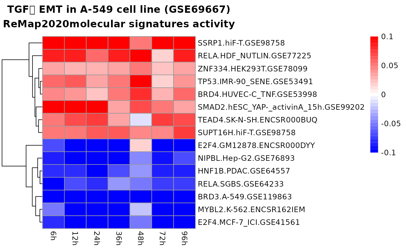
  nfolds = 5)

Exploring results

top_signatures <- head(res_rna_seq$results$remap, 15)
pheatmap::pheatmap(
  mat = top_signatures[, 2:8],
  labels_row = top_signatures$name,
  cluster_cols = FALSE,
  color = colorRampPalette(c("blue", "white", "red"))(35),
  breaks = seq(from = -0.1, to = 0.1, length.out = 36),
  main = "TGFꞵ EMT in A-549 cell line (GSE69667)\nReMap2020molecular signatures activity"
)

Microarray data

Obtaining the expression data

Here, we have downloaded supplementary data file containing pre-processed data from GSE17708 study. This supplementary file is an xls file that needs to be loaded to R and converted into matrix before we can use it.

Ready to use “counts” matrix (these are not raw counts) can be downloaded from our server.

download.file(url = "https://zdglab.iimcb.gov.pl/mmigdal/GSE17708.rda", 
              destfile = "GSE17708.rda")
load("GSE17708.rda")

knitr::kable(head(counts_microarray))

	0hr_1	0hr_2	0hr_3	0.5hr_1	0.5hr_2	0.5hr_3	1hr_1	1hr_2	1hr_3	2hr_1	2hr_2	4hr_1	4hr_2	4hr_3	8hr_1	8hr_2	8hr_3	16hr_1	16hr_2	16hr_3	24hr_1	24hr_2	24hr_3	72hr_1	72hr_2	72hr_3
780	14	14	14	14	14	15	14	14	15	15	14	15	15	15	16	15	16	16	16	16	15	15	16	15	15	15
5982	7	6	6	6	6	6	6	6	6	6	6	6	6	6	6	6	6	6	6	6	6	6	6	6	6	6
3310	5	5	4	4	4	4	4	4	4	5	5	4	4	4	4	4	4	5	4	4	5	5	4	5	5	5
7849	20	19	20	20	20	20	19	19	19	20	19	19	20	19	19	19	19	19	19	19	19	19	20	19	19	19
2978	7	7	7	7	7	7	7	7	7	7	7	7	7	7	7	7	7	7	7	7	7	7	7	7	7	7
7318	5	5	5	5	5	5	5	5	5	5	5	5	5	5	5	5	5	5	5	5	5	5	5	5	5	5

Constructing experiment design

Again we construct design matrix, by taking advantage of the patterns present in the sample names.

cond <- sub(pattern = "_.*", replacement = "", x = colnames(counts_microarray))
ncond <- cond %>% unique() %>% length()
design <- diag(ncond)[rep(seq_len(ncond), times = table(cond)[unique(cond)]), ]
rownames(design) <- colnames(counts_microarray)
colnames(design) <- unique(cond)

knitr::kable(design)

	0hr	0.5hr	1hr	2hr	4hr	8hr	16hr	24hr	72hr
0hr_1	1	0	0	0	0	0	0	0	0
0hr_2	1	0	0	0	0	0	0	0	0
0hr_3	1	0	0	0	0	0	0	0	0
0.5hr_1	0	1	0	0	0	0	0	0	0
0.5hr_2	0	1	0	0	0	0	0	0	0
0.5hr_3	0	1	0	0	0	0	0	0	0
1hr_1	0	0	1	0	0	0	0	0	0
1hr_2	0	0	1	0	0	0	0	0	0
1hr_3	0	0	1	0	0	0	0	0	0
2hr_1	0	0	0	1	0	0	0	0	0
2hr_2	0	0	0	1	0	0	0	0	0
4hr_1	0	0	0	0	1	0	0	0	0
4hr_2	0	0	0	0	1	0	0	0	0
4hr_3	0	0	0	0	1	0	0	0	0
8hr_1	0	0	0	0	0	1	0	0	0
8hr_2	0	0	0	0	0	1	0	0	0
8hr_3	0	0	0	0	0	1	0	0	0
16hr_1	0	0	0	0	0	0	1	0	0
16hr_2	0	0	0	0	0	0	1	0	0
16hr_3	0	0	0	0	0	0	1	0	0
24hr_1	0	0	0	0	0	0	0	1	0
24hr_2	0	0	0	0	0	0	0	1	0
24hr_3	0	0	0	0	0	0	0	1	0
72hr_1	0	0	0	0	0	0	0	0	1
72hr_2	0	0	0	0	0	0	0	0	1
72hr_3	0	0	0	0	0	0	0	0	1

Translating gene symbols into FANTOM5 core promoters

Next, we need to translate expression matrix’s row IDs to FANTOM5 core promoters. The only difference is that this time we map ENTREZ IDs to FANTOM5 promoters.

eh <- ExperimentHub::ExperimentHub()

## snapshotDate(): 2022-10-31

entrez2fantom <- eh[["EH7699"]]

## see ?xcoredata and browseVignettes('xcoredata') for documentation

## downloading 1 resources

## retrieving 1 resource

## loading from cache

counts_fantom <- translateCounts(counts_microarray, dict = entrez2fantom)

Processing the counts and molecular signatures

Here, our workflow deviates from the previous example. Because, we use the pre-processed expression data we don’t really want to normalize it. Instead we will use the data as is.

mae_microarray <- regressionData(
  expr_mat = counts_fantom,
  design = design,
  base_lvl = "0hr"
)

selected_signatures <- c(
  "SSRP1.hiF-T.GSE98758", "BRD3.A-549.GSE119863", "RELA.HDF_NUTLIN.GSE77225", 
  "SMAD2.hESC_YAP-_activinA_15h.GSE99202", "TET2.Jurkat.GSE85524", "SUPT16H.hiF-T.GSE98758", 
  "E2F4.MCF-7_ICI.GSE41561", "HNF1B.PDAC.GSE64557", "TP53.IMR-90_SENE.GSE53491", 
  "MBD2.HeLa.GSE41006", "E2F4.GM12878.ENCSR000DYY", "TEAD4.SK-N-SH.ENCSR000BUQ", 
  "BRD4.HUVEC-C_TNF.GSE53998", "NIPBL.Hep-G2.GSE76893", "BRD4.HUVEC-C_TNF_JQ1.GSE53998", 
  "BRD4.HUVEC-C_modGFP.GSE93030", "RELA.SGBS.GSE64233", "MYBL2.K-562.ENCSR162IEM", 
  "RBPJ.GSC8-11.GSE74557", "ZNF334.HEK293T.GSE78099")
mae_microarray <- addSignatures(mae_microarray, 
                                remap = remap_promoters_f5[, selected_signatures])
mae_microarray <- filterSignatures(mae_microarray, min = 0.05, max = 0.95)

Modeling gene expression

# register parallel backend
doMC::registerDoMC(cores = 5L)

# set seed
set.seed(314159265)

res_microarray <- modelGeneExpression(
  mae = mae_microarray,
  xnames = "remap",
  nfolds = 5)

Exploring results

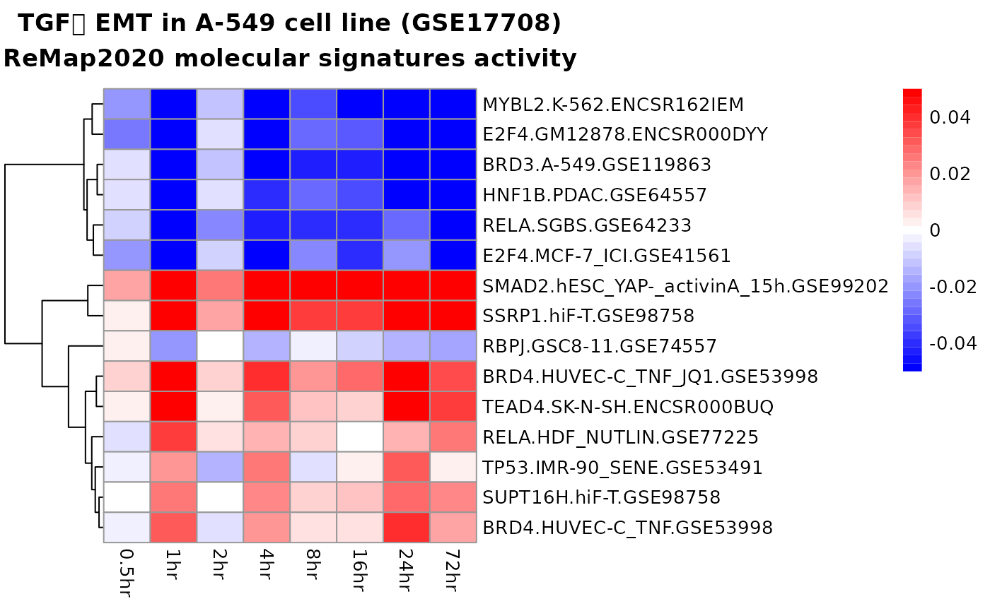
top_signatures <- head(res_microarray$results$remap, 15)
pheatmap::pheatmap(
  mat = top_signatures[, 2:9],
  labels_row = top_signatures$name,
  cluster_cols = FALSE,
  color = colorRampPalette(c("blue", "white", "red"))(35),
  breaks = seq(from = -0.05, to = 0.05, length.out = 36),
  main = "TGFꞵ EMT in A-549 cell line (GSE17708)\nReMap2020 molecular signatures activity"
)

Migdal

2/15/2022

Introduction

RNA-seq data

Obtaining the expression data

Constructing experiment design

Obtaining core promoters annotation and molecular signatures

Translating gene symbols into FANTOM5 core promoters

Processing the counts and molecular signatures

Modeling gene expression

Exploring results

Microarray data

Obtaining the expression data

Constructing experiment design

Translating gene symbols into FANTOM5 core promoters

Processing the counts and molecular signatures

Modeling gene expression

Exploring results